Saturation in metal Binder Jetting: Simple in principle, complicated in practice?

Saturation, for the uninitiated, is the primary driving variable used when executing the manufacturing step required to make ‘green’ parts in Binder Jetting (BJT). It is simple to understand in principle, but can be difficult to understand when reducing principle to practice. This article will introduce several concepts key to understanding Binder Jetting technology’s #1 variable, including:

• The absolute basic steps of BJT Additive Manufacturing
• What saturation is and some basic units of measure
• What voxels are and how they are defined
• Binder nozzle geometries and how they relate to voxels
• Control options and how choices in controls affect saturation options.

A Binder Jetting primer

BJT Additive Manufacturing is a fast-growing manufacturing technology that is finding increasing uses in the Metal Injection Moulding industry, from the production of low-quantity prototypes to high-volume products.

Like all Additive Manufacturing, this is a layer-based AM process and parts are built up one layer at a time, in this case by binding layers of powder together in a build box. A complete process for creating a finished, dense part usually consists of manufacturing, curing, depowdering, and sintering. There are many articles explaining the workflow, so this article will focus on the manufacturing step.

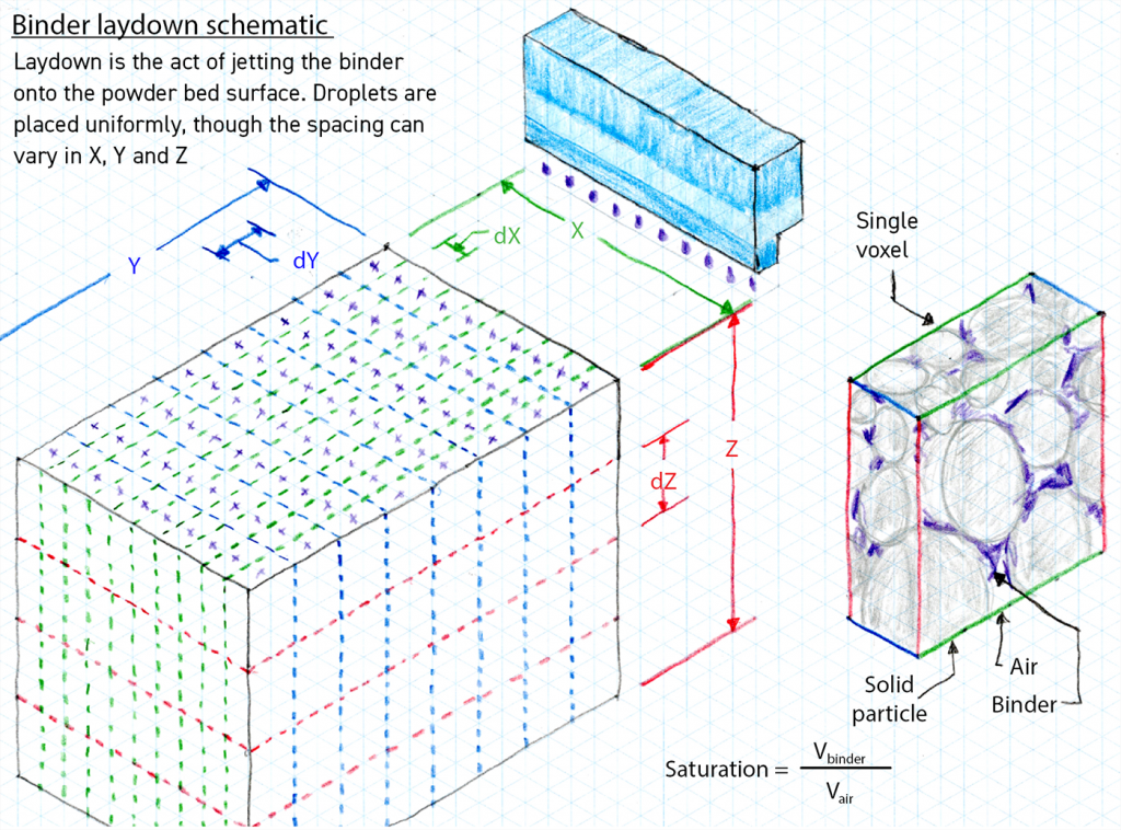
As illustrated in Fig. 2, three basic operations are repeated inside a typical Binder Jetting machine during manufacturing:b

• Spread a uniform layer of powder
• Additively manufacture an image in binder that represents the cross-section of the part at that layer height
• Add some amount of energy, usually heat, to slightly dry the surface

These three activities happen repeatedly, from the bottom to the top. The engineering complexity of any Binder Jetting machine is much larger than what I have described, but this is the essence. The rest of this article is meant to describe how the machine decides where to place the binder droplets and how much gets used in the build.

Saturation defined

Let us get the easy part out of the way and start with the basic definition of saturation and its underlying assumptions. Of the latter, the most important is that the powder we are binding is made of whole granules and that these are insoluble in the binder being jetted as the glue. This is true for 99% of metal BJT, as the binder is not normally mixed into the powder, but it is not true for several other forms of BJT, nor when binding some agglomerates. This discussion will only lightly describe variable-sized drops, as they are an emerging laydown strategy.

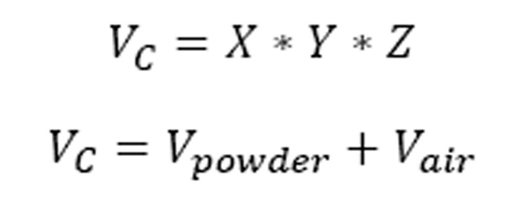
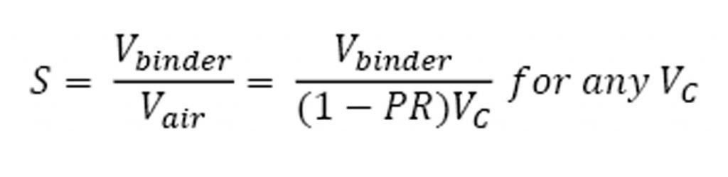
Given a contained volume of powder VC with dimensions X,Y,Z, we can say the container is filled with solid granules and air. That is,

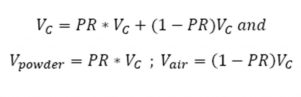
We can introduce the term ‘Packing Rate’, PR, to express the ratio of the measured powder density to the material’s solid density, and rewrite.

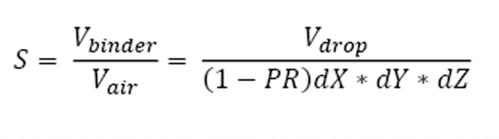
If we fill Vair with some volume of binder, Vbinder, we can define saturation, S.

This bulk property of saturation is true all the way down to the base unit level: the Voxel – I love this word, I have to say. It means Volumetric Picture Element. This is the most accurate and descriptive word that has been coined in a long time. It is one ‘dot’ in a picture, extruded through some thickness. It is perfect. In Fig. 3, you can see this principle at work. For the typical BJT machine, the volume is broken down into discrete, fractional pieces. These cubic shapes can be of any size, ratiometrically, and, in most cases, X ≠ Y ≠ Z.

One needs to be familiar with a few terms not common in manufacturing processes. A BJT machine is often rated by the unit DPI, or Dots Per Inch. BJT follows 2D printing technology and, since much of that is based on typographic printing, it continues to be based on the old system of units ‘points’ and ‘picas’. You will often (though not always) see multiples of 6, 12, and 72 DPI.

DPI and Droplet Spacing are inverts, typically converted from inches to microns. The equation is a simple one:

Print density in DPI

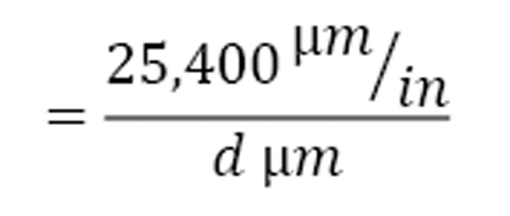
where d is the distance between drops

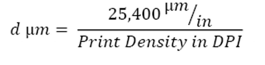
where DPI is the rated build density

You might see ‘accuracy’ listed in a machine specification as a number, like 63.5 µm. Using the equation, we can see this spacing describes a 400 DPI process. This is invertible and any distance can be used as a basis for a DPI (that is, if you have 1.016mm between dots, you could call it 25 DPI).
With this as background, we can take any volume VC and decompose it to a combination of voxels

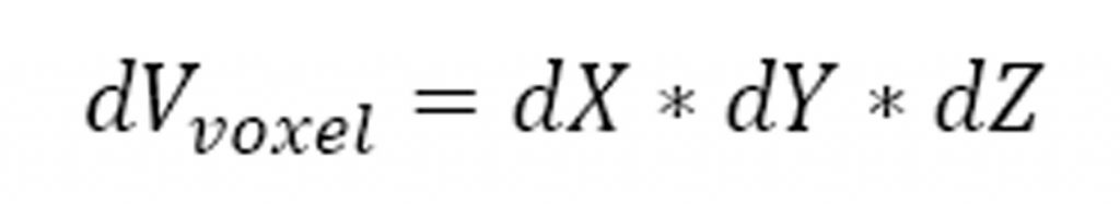
Where dX is the X spacing between drops, dY is the Y spacing between drops, and dZ is the Z spacing between drops. We can say that each voxel is additively manufactured with one droplet of binder with volume Vdrop. With these new variables, we can rewrite the fundamental saturation equation:

It is easy enough to understand that dZ is the layer thickness and it is easy enough to imagine a way to measure the droplet’s volume. Where the confusion comes is understanding where dX and dY come from and how a machine computes them. To understand that, we need to understand real-world inkjet Binder Jetting modules.

Before I get too far in, though, it is important to understand two things:

• This is just algebra! This is not physics!
• Since it is just algebra, the equations can be easily manipulated

By ‘not physics’, I mean that this math cannot be used for things like simulations or making predictions about the interactions between a fluid and a powder, even when the physical properties of everything are known. These simple equations do not account for the real wetting phenomenon of the process. It is a short-hand method for relating the Additive Manufacturing strategy.

It is also based on volumes, not mass. Measuring volume is notoriously less precise than measuring weights, but, in this case, the percentages would feel strange to control. Saturation as a relationship between the volume of binder and volume of air in the powder is easy to understand and envision. This is especially true when moving between powder types.

Over the years, I have found that saturation does not generally vary a great deal and it is usually between 50-75%. Also, it is as true when additively manufacturing light materials like silica with non-reactive binders as it is when additively manufacturing denser materials like tungsten alloys. Likewise, most powders do not seem to vary that much by packing rate either, with a normal range of 50-60% solid. There are outliers, like sands and more filamentary particles, but, by and large, this is common.
If someone used mass ratio as the primary relationship expressing binder deposition rates to the mass of the voxel, they might be misled into thinking they are consuming much more binder in one case than the other. And the ‘feel’ for the consumption would be backwards.

For example, silicon carbide has a normal density of 3.21 g/cm3. If you had a 55% dense powder additively manufactured at a saturation rate of sixty percent and back-calculate with a binder density of 1.05 g/cm3, you would be applying binder at the rate of 13.8% by mass.

But, if you were additively manufacturing tungsten carbide, with a density closer to 15.6 g/cm3, the same rate would be 3.3% by mass. And paradoxically, if you increase saturation to 80%, the mass ratio would only increase to 4.2%. It would be easy to think, at first glance, that the tungsten carbide was consuming less binder, when, in fact, it is not. Using volume ratios allows consumption rates to be compared consistently across different powder types more easily for the user.

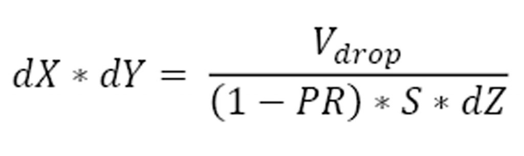
We often want to compute the pair dX and dY, given a desired saturation, a specified layer thickness, and a known powder packing rate. Here is the secret: it is as simple as rewriting the equation and understanding the constraints on dX and dY.

This is where it starts to get confusing. To the user/operator, the number pairs for dX and dY can seem to come from nowhere, but, in fact, they are driven by two things: the physical layout of the jetting module(s) and the complexity of the controls available. To illustrate this, consider the Polaris PQ-512/85AAA module from FujiFilm Dimatix, shown in Fig. 4.

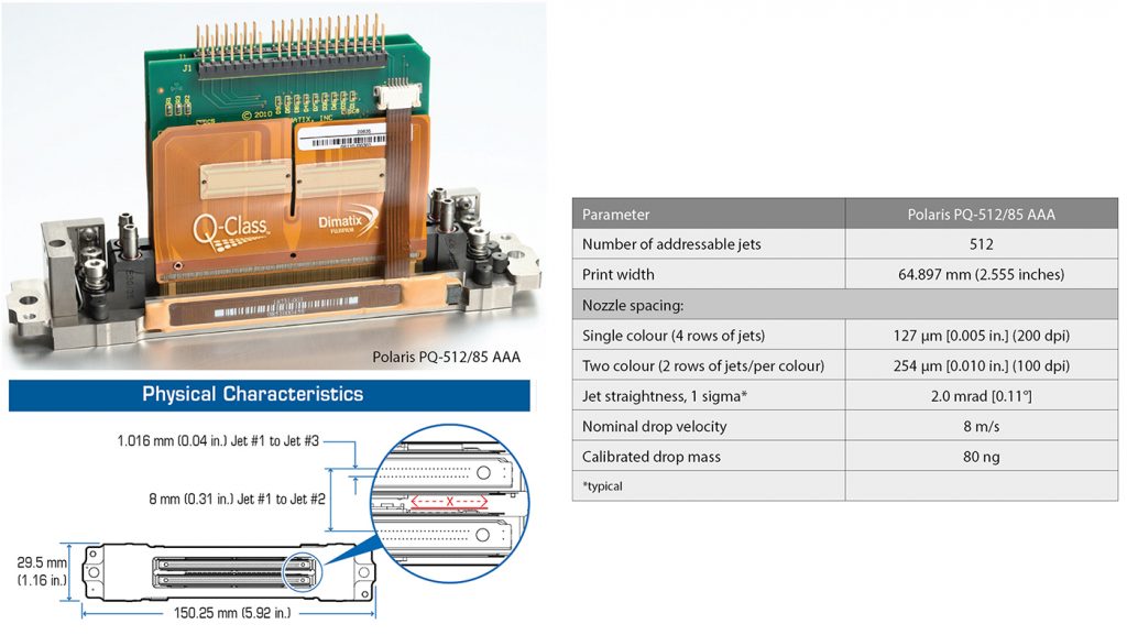
Though they could be assigned either way, X is generally defined as the axis in line with the nozzles, while Y is defined as the spacing between the jetted lines. In this example, the native dX spacing would be 127 microns (200 DPI), but dY will require more explanation.

The first constraint a typical BJT machine will place on the calculations is that they all must involve ‘whole drops’ and ‘whole voxels’. For dX, it means we can only divide the spacing by an integer (or multiply the DPI by an integer) to achieve a new dX spacing. Practically, this means you can additively manufacture with spacings of 127 µm, 63.5 µm, 42.33 µm, etc., but you cannot choose 50 µm exactly.

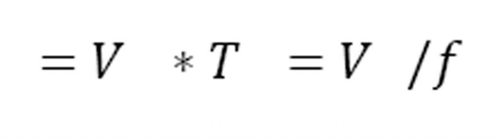
You will find that, with most piezo-driven binder nozzles, there is an interplay and relationship between jetting frequency, droplet volume, and droplet velocity. Because of this, most machines are designed to additively manufacture by jetting with a constant frequency while moving the head at a constant velocity (Fig. 5). The resulting spacing, dY, is thus the build velocity times the jetting period.

Mechanically, the same integer divider rule still applies vis-à-vis drop spacing. This example is challenging, as the intra-row spacing and the row-to-row spacing are not evenly divisible. The former, at 1.016 mm, means it has a native Y resolution of 25 DPI. But the second row is spaced at 8 mm (3.175 DPI), and these do not mix. No single DPI can be used that will allow the head to be fired as a complete unit, while also perfectly aligning every drop.

As an aside, this highlights one of the difficulties designers face when implementing binder nozzle controllers. Though it is not entirely apparent, a 2D printing matrix like the one shown here can often be controlled by firing each line of piezos independently, or in groups. However, this approach would require as many pulse generators and data-paths as the designer wants line-level control. It is a true ‘value engineering’ question.

For the sake of an example, let us specify a laydown of 200 DPI x 200 DPI and accept that the saturation value would be correct. It means that there would be 62.992 DROPS between row 1 and row 3. So if nozzle one drops at position = 0, nozzle two, 63 drops later, will drop at 0.001 mm, with a persistent .001 mm error in absolute drop placement in every line. The error is non-cumulative, but it is ever- present. For our purposes, we shall ignore it, but if this fine level of control were required for an application, at least two generators would be needed.

On the flip-side, though, if the decision was made to control all four lines independently, the value for dY would be nearly free-settable within the bounds of saturation. That is because you could always come up with a combination of position tracking and timing offsets to achieve (nearly) perfect spacing.

All that said, for the purpose of this discussion, we shall say DPIX must be DPImXi where i is the number of passes. For this module, we shall use DPImX=200 DPI. DPIY must be DPImYj and DPIY will further be constrained by the frequency/velocity relationship. For this module, we shall use DPImY = 25DPI. With everything defined, the control software now starts computing dX and dY pairs to find the best fit.

At this step, the control system is looking primarily at the aspect ratio of the drop placement and it is using exact dY values instead of constrained ones. dY will be adjusted in the final calculation, but what the software examines first is the voxel aspect ratio.

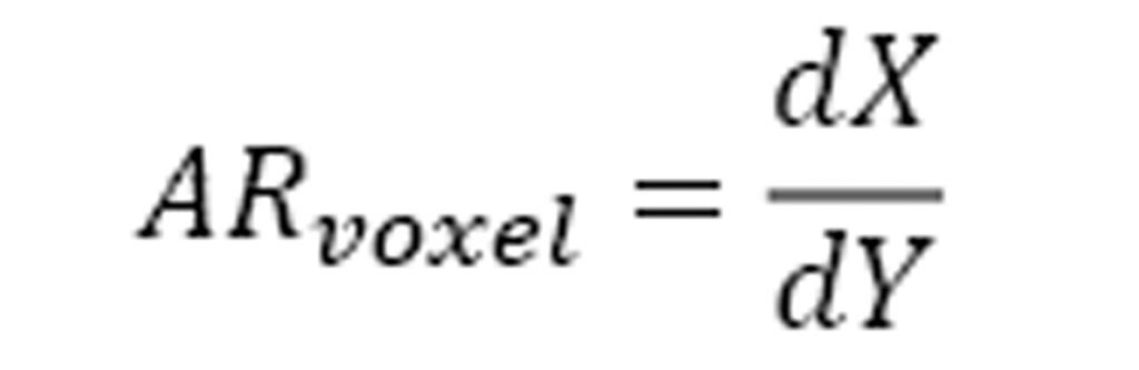
A good BJT process will try to operate as close to 1 as possible. In the example shown in Table 1, the software should pick option two. With two passes selected, the software will now rectify the dY value. In this case, the Binder Jetting could be done with either 500 DPI or 525 DPI, both of which are detailed in Table 2.

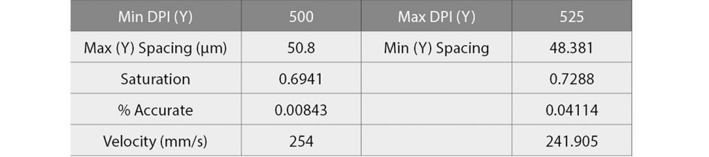
Obviously, 500 DPI is closer to 504 than 525, so the former would be chosen. And that is it. The real saturation would be 69.4% and the machine would configure itself to build with a speed of 254 mm/s and a jetting frequency of 5 kHz. The final process will have resolutions 400 DPI (X) x 500 DPI (Y) x 338.7 DPI (Z). That translates to a neatly stacked grid of voxels with size 63.5 x 50.8 x 75 µm.

Though this is a contrived example with somewhat invented numbers, this is how a Binder Jetting machine works. While saturation is just a number, and the actual physics involved with Additive Manufacturing are much more complex than this suggests, strict control of it has proven to be a reliable method of achieving your best results for over twenty years.

One last thing that should be noted about this simple calculation: accurately measuring and tracking the ‘as-manufactured’ packing rate is key. The ballistic impact of the binder on the powder causes it to rearrange in most cases, if not all. A good starting point for approximation is 90–95% of the measured tap-density, but, once you are making samples, you have to check and adjust accordingly.

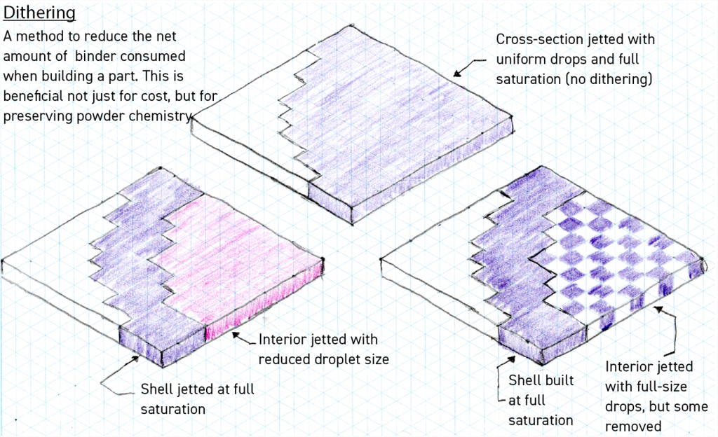
Bonus: Dithering

Dithering the build has long been an established method of controlling print density in 2D applications. By dithering the drops, the machine seeks to minimise the chance of excess bleed of the ink, while still preserving the original image quality.

In Binder Jetting, dithering is done for the same reason, but, with BJT, you get an additional benefit: any chemical that is added to the binder has the potential to be added to the chemistry of the final part. If it cannot burn out cleanly in the furnace, or during the curing step, those residuals can affect the material properties of your part. The most affected chemical is carbon, as almost all binders are based on polymers with a carbon backbone.

Most dithering strategies fall into one of two categories: using different sized drops for the interior and exterior or using all the same sized drops, but removing some. In both cases, an outer shell of some voxel thickness is additively manufactured with full saturation, as we calculated earlier. This guarantees the part can be handled post-cure.

In the case of drops of multiple sizes, the machine takes advantage of binder nozzle flexibility. Most nozzle modules can generate a few different sized drops from a single type, so a smaller-sized drop might be selected to uniformly fill the interior. For droplet reduction when using standard drops, special filtering algorithms are employed to optimise the infill. Both methods achieve the same goal, in that less binder is used.

It is important to note that dithering is only possible when using binder nozzles with the right controls, and/or a software stack that supports directly working on voxels. Again, this is value engineering at work. To have the feature, you have to pay for the feature.

I hope you found this article useful and informative. If you still have questions about how to tune your machine and process, please reach out!

Author

Dan Brunermer
B-jetting llc.
124 Grant Avenue Suite 110, Vandergrift, Pennsylvania 15690,
USA

[email protected]
[email protected]
www.b-jetting.com